


Ever wondered what is the sound absorption of your absorber in situ?
SONOCAT
A multifunctional acoustic device for in-situ measurements.
Sound absorption of a material can now be measured in the field. It is well known that, normally, sound absorption measurement needs to be done in a reverberant sound field and controlled environment such as a reverberation chamber referred to the traditional method, for example, ISO 354. The reason is the measurement method relies on the sound field inside a reverberation chamber which cannot be obtained in situ.
Sonocat measures 3D sound waves, meaning that the equipment can distinguish between the incident wave, reflected wave, and the total or the active sound wave. This overcomes the limit of relying on the sound field when measuring sound absorption and sound transmission loss, allowing the acousticians to investigate these acoustic parameters in the field.
Sonocat can be useful in many cases, for example, when the test object cannot fit in the facilities or when it’s already installed at the site. Imagine a noise barrier that has been next to the highway for ten years, and the acoustic engineer needs to inspect whether the performance is still well-maintained. It won’t be possible to move the barrier to a lab, this is when in-situ measurement devices become handy. The engineer will be able to inspect the current performance of the absorption material inside the barrier as well as the sound transmission loss of the barrier, they can also use this to study the life span and plan for their next maintenance.
With the capability of measuring 3D sound waves, Sonocat can also be used to locate the sound source or the leakage point. This can be useful for those who work in the automotive industry, for example, inspecting the vehicle to find the correct spot that causes noise intrusion problems and deciding the most effective solution.


Most industrial activities create noise that can be harmful to the environment as well as to their workers. To minimize this effect, governments, associations, and companies have created regulations, standards, and codes to set the allowable noise both inside the sites, that can be harmful to the workers, as well as to the environment. In a lot of cases, during the planning phase, the plant owner and project management want to be sure that the noise levels are acceptable. Since the plant is not built yet, what can be done is creating a noise model to simulate the plant, so that the noise levels can be predicted. In this article, we will explore how we can do so.
The first thing we must know is how much noise does the noise sources inside of the plant will emit. The noise source is usually described in two ways which is Sound Power Level (Lw or SWL), and Sound Pressure Level (Lp or SPL) in certain distance, most commonly Lp in 1 m distance. There are multiple ways to get this information for certain noise sources. First, if the equipment type and model have been chosen, the equipment manufacturer will normally report the noise level in their datasheet. However, this is not usually the case with most of noise predictions since the noise study is normally done before the equipment suppliers are appointed. So, the second way to be able to predict the noise emission is by following empirical formulas that are developed by researchers. You can find such formulas in some textbooks, journals, and papers. For rotating parts, you will need its rated power and rotational speed to be able to estimate the noise emission.
For example, in the speed range of 3000-3600 rpm, the noise level of a pump with drive motor power above 75 kW can be predicted using the following equation:

Suppose a pump with rotational speed of 3000 rpm and 100 kW, according to the formula, it can be estimated that the noise level at 1 m from the pump would be 92 dB. And suppose the noise source can be considered as point source on the ground (hemisphere propagation), the sound power level of the pump can be calculated using the following formula:

Where r is the distance from source to receiver
And in this case, the predicted Lw would be 100 dB.
Thirds, noise measurement to a similar equipment can also be an option to be able to determine the noise level of the new equipment. Another option, in some countries, there are noise emission limit for certain equipment, you can use that limit if it is applicable for your project.
After the Lw of all noise sources is obtained, we want to calculate the noise levels (the Lp) at the receivers. There are some standards which procedure can be followed to calculate this. Few of which are ISO 9613-2, NORD 2000, CNOSSOS EU, and many others. Most of the standards consider some factors to the calculation such as distance, atmospheric absorption, ground reflection, screening effect (from barriers and obstacles) and other factors such as volume absorption from vegetation, industrial site, etc. Most consultants and projects will require a software such as SoundPLAN to do this calculation.
Depending the project, there are few types of noise limit which compliance will need to be ensured. The most common ones are environmental noise limit, noise exposure limit, area noise limit and absolute noise limit. Besides, the noise level during emergency is also modelled so that the information can be used for safety and PAGA (Public Address and General Alarm) study.
Environmental noise limit is usually calculated for the plant’s contribution to the plant’s boundary as well as to the nearest sensitive receiver such as residential and school near the plant. How this is accessed depends on the regulation applicable on the plant area. In Indonesia for example, the noise limit for residential area is Lsm 55 dBA and industrial area is Lsm 70 dBA. Lsm is a measure like Ldn, but the night noise level addition is 5 dB instead of the 10 dB addition that most other countries, especially Europeans use. To ensure compliance with this regulation, the noise level at fence should be less than Lsm 70 dBA, and suppose there is a residential area nearby, the contribution from the site should be less than 55 dBA. It is also advisable to measure the existing noise level at the sensitive receivers to make the study more relevant to the situation.
Noise exposure limit is the maximum exposure to noise that the workers get during their working period. In Indonesia, the noise exposure limit is 85 dBA for 8 working hours. To change the working hours, 3 dB exchange rate is used. For example, if the noise level in the plant is 88 dBA, then the workers can only work there for 4 hours, if it is 91 dBA, then the time limit is 2 hours, and so on. To extend the working hours on a noisy area, the options are to actually reduce the noise level by reducing the noise emission from the source or noise control at transmission (for example using barrier), or by usage of Hearing Protection Device (HPD) for the workers such as ear plugs and ear muffs. The noise exposure of workers after usage of HPD can be calculated using the following formula:

Where NRR is the noise reduction rating of the HPD in dB.
Different area might have different noise level limits, and therefore area noise limits are useful. For example, in an unmanned mechanical room, the noise level can be high, for instance 110 dBA. However, inside of the site office, the allowable noise level is much lower, for example 50 dBA. This noise level shall be calculated to ensure compliance with the noise limit. Different companies might have different limits for this to ensure their employees’ health and productivity. If the area is indoor and the noise source is outdoor, then the interior noise level can be estimated using standards such as ISO 12354-3.
The absolute noise limit is the highest noise level allowable at the plant, and shall not be exceeded at any times, including emergency. In most cases, the absolute noise limit for impulsive sound is 140 dBA. To ensure compliance with this requirement, potential high-level noise shall be calculated, for example safety valves.
During emergency, different noise sources than normal situation will be activated, such as flare, blowdown valves, fire pumps, and other equipment. In such cases, the sound from the alarm and Public Address system must be able to be heard by the workers inside of the plant. Normally the target for the SPL from the PAGA system should be higher than 10 dB above the noise level. Therefore, the noise level during emergency in each area should be well-known.
Geonoise just made basic noise calculations even easier.
You can make free calculations online to add, subtract decibel levels, calculate NR values and make your own reverberation calculations online!
Free noise calculations online

Rail transport or train transport is one of the main transportation modes these days, both for transferring passengers and goods. Every day people commute to work and back home using trains in a form of subway systems, light rail transits and other types of rail transport. These types of system can create noise both to the passengers inside of the train as well as to the environment. In this article, we will discuss about noise source components that we hear daily both inside and outside of the train.
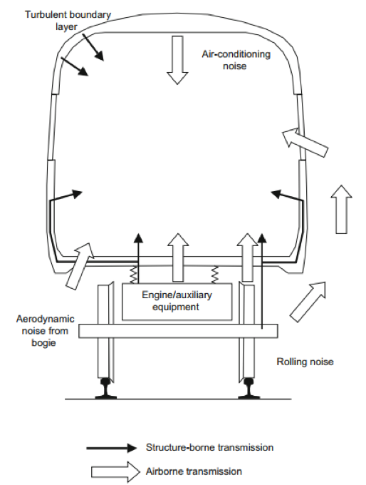
If we pay attention to the noise when we are on board of a train, there are more than one noise source that we can hear. The main sources for interior noise in a train are turbulent boundary layer, air conditioning noise, engine/auxiliary equipment, rolling noise and aerodynamic noise from bogie, as illustrated in the following figure.
By the way, we wrote and recorded the sound of Jakarta MRT. You can see the link below to help you imagine the train situation better.
Exploring Jakartan Public Transportation Through The Sound
Rolling noise is caused by wheel and rail vibrations induced at the wheel/rain contact and is one of the most important components in railway noise. This type of noise depends on both wheel and rail’s roughness. The rougher the surface of both components will create higher noise level both inside and outside of the train. To be able to estimate the airborne component from the rolling noise, we must consider wheel and track characteristics and roughness.
Another noise component that contributes a lot to railway noise is aerodynamic noise which can be caused by more than one sources. These types of sources may contribute differently to internal noise and external noise. For example, aerodynamic noise contributes quite significantly at lower speeds to internal noise while for external noise, it doesn’t contribute as much if the train speed is relatively low. For example, on the report written by Federal Railroad Administration (US Department of Transportation), it is stated that aerodynamic sources start to generate significant noise at speeds of approximately 180 mph (around 290 km/h). Below that speed, only rolling noise and propulsion/machinery noise is taken into consideration for external noise calculation. In addition to external noise, machinery noise also contributes to the interior noise levels. This category includes engines, electric motors, air-conditioning equipment, and so on.
To perform the measurements of railway noise, there are several procedures that are commonly followed. For measurement of train pass-by noise, ISO 3095 Acoustics – Railway applications – measurement of noise emitted by rail bound vehicles, is commonly used. This standard has 3 editions with the first published in 1975, and then modified and approved in 2005 and again in 2013. The commonly used measures for train pass-by are Maximum Level (LAmax), Sound Exposure Level (SEL) and Transit Exposure Level (TEL).
For interior noise, the commonly used test procedure is specified in ISO 3381 Railway applications – Acoustics – Measurement of noise inside rail bound vehicles. This procedure specifies measurements in few different conditions such as measurement on trains with constant speed, accelerating trains from standstill, decelerating vehicles, and stationary vehicles.
Written by:
Hizkia Natanael
Acoustical Design Engineer
Geonoise Indonesia
hizkia@geonoise.asia
Reference:
D. J. Thompson. Railway noise and vibration: mechanisms, modelling and means of control. Elsevier, Amsterdam, 2008
Federal Railroad Administration – U.S. Department of Transportation, High-Speed Ground Transportation Noise and Vibration Impact Assessment. DOT/FRA/ORD-12/15. 2012